Basic Equations¶

We consider a constant-property slab of atoms, located at a height \(h\) above the visible solar “surface”, in the presence of a deterministic magnetic field of arbitrary strength \(B\), inclination \(\theta_B\) and azimuth \(\chi_B\) (see Fig. 1). The slab’s optical thickness at the wavelength and line of sight under consideration is \(\tau\). We assume that all the atoms inside this slab are illuminated from below by the photospheric solar continuum radiation field, whose center-to-limb variation has been tabulated by Pierce (2000). The ensuing anisotropic radiation pumping produces population imbalances and quantum coherences between pairs of magnetic sublevels, even among those pertaining to the different \(J\)-levels of the adopted atomic model. This atomic level polarization and the Zeeman-induced wavelength shifts between the \(\pi\) (\(\Delta{M}=M_u-M_l=0\)), \(\sigma_{\rm blue}\) (\(\Delta{M}=+1\)) and \(\sigma_{\rm red}\) (\(\Delta{M}=-1\)) transitions produce polarization in the emergent spectral line radiation.

In order to facilitate the understanding of the code, in the following we summarize the basic equations which allow us to calculate the spectral line polarization taking rigorously into account the joint action of atomic level polarization and the Hanle and Zeeman effects. To this end, we have applied the quantum theory of spectral line polarization, which is described in great detail in the monograph by Landi degl’Innocenti & Landolfi (2004). We have also applied several methods of solution of the Stokes-vector transfer equation, some of which can be considered as particular cases of the two general methods explained in §6 of Trujillo Bueno (2003).

<<<<<<< HEAD .. _image_geometry:

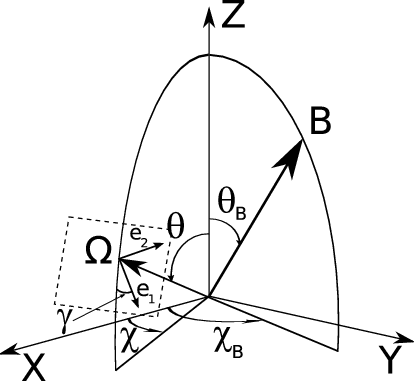
The \(Z\)-axis is placed along the vertical to the solar atmosphere. The magnetic field vector, \(\mathbf{B}\), is characterized by its modulus \(B\), the inclination angle \(\theta_B\) and the azimuth \(\chi_B\). The line-of-sight, indicated by the unit vector \(\mathbf{\Omega}\), is characterized by the two angles \(\theta\) and \(\chi\). The reference direction for Stokes \(Q\) is defined by the vector \(\mathbf{e}_1\) on the plane perpendicular to the line-of-sight. This vector makes an angle \(\gamma\) with respect to the plane formed by the vertical and the line-of-sight. In the figures showing examples of the emergent Stokes profiles, our choice for the positive reference direction for Stokes \(Q\) is \(\gamma=90^\circ\), unless otherwise stated. For off-limb observations, we have \(\theta=90^\circ\), while for observations on the solar disk, we have \(\theta<90^\circ\). Note also that \(\chi\) is generally taken to be \(0^\circ\).

The radiative transfer approach¶

The emergent Stokes vector \(\mathbf{I}(\nu,\mathbf{\Omega})=(I,Q,U,V)^T\) (with \(^T\)=transpose, \(\nu\) the frequency and \(\mathbf{\Omega}\) the unit vector indicating the direction of propagation of the ray) is obtained by solving the radiative transfer equation

\[\frac{d}{ds}\mathbf{I}(\nu,\mathbf{\Omega}) = \mathbf{\epsilon}(\nu,\mathbf{\Omega}) - \mathbf{K}(\nu,\mathbf{\Omega}) \mathbf{I}(\nu,\mathbf{\Omega}), \label{eq:rad_transfer}\]

where \(s\) is the geometrical distance along the ray under consideration, \(\mathbf{\epsilon}(\nu,\mathbf{\Omega})=({\epsilon}_I,{\epsilon}_Q,{\epsilon }_U,{\epsilon}_V)^T\) is the emission vector and

\[\begin{split}\mathbf{K} = \left( \begin{array}{cccc} \eta_I & \eta_Q & \eta_U & \eta_V \\ \eta_Q & \eta_I & \rho_V & -\rho_U \\ \eta_U & -\rho_V & \eta_I & \rho_Q \\ \eta_V & \rho_U & -\rho_Q & \eta_I \end{array} \right) \label{eq:propagation}\end{split}\]

is the propagation matrix. Alternatively, introducing the optical distance along the ray, \({\rm d}{\tau}=-{\eta_I}{\rm d}s\), one can write the Stokes-vector transfer Eq. ([eq:rad_transfer]) in the following two ways:

The first one, whose formal solution requires the use of the evolution operator introduced by Landi degl’Innocenti & Landi degl’Innocenti (1985), is

\[{{d}\over{d{\tau}}}{\bf I}\,=\,{\bf K}^{*} {\bf I}\,-\,{\bf S}, \label{eq:rad_transfer_peo}\]

where \({\bf K}^{*}={\bf K}/{\eta_I}\) and \({\bf S}=\mathbf{\epsilon}/{\eta_I}\). The formal solution of this equation can be seen in eq. (23) of Trujillo Bueno (2003).
The second one, whose formal solution does not require the use of the above-mentioned evolution operator is Rees et al. (1989)

\[{{d}\over{d{\tau}}}{\bf I}\,=\,{\bf I}\,-\,{\bf S}_{\rm eff}, \label{eq:rad_transfer_delo}\]

where the effective source-function vector \(\,{\bf S}_{\rm eff}\,=\,{\bf S}\,-\, {\bf K}^{'}{\bf I},\,\,\,\) being \(\,{\bf K}^{'}={\bf K}^{*}-{\bf 1}\) (with \(\bf 1\) the unit matrix). The formal solution of this equation can be seen in eq. (26) of Trujillo Bueno (2003).

Once the coefficients \(\epsilon_I\) and \(\epsilon_X\) (with \(X=Q,U,V\)) of the emission vector and the coefficients \(\eta_I\), \(\eta_X\), and \(\rho_X\) of the \(4\times4\) propagation matrix are known at each point within the medium it is possible to solve formally Eq. ([eq:rad_transfer_peo]) or Eq. ([eq:rad_transfer_delo]) for obtaining the emergent Stokes profiles for any desired line of sight. Our computer program considers the following levels of sophistication for the solution of the radiative transfer equation:

Numerical Solutions. The most general case, where the properties of the slab vary along the ray path, has to be solved numerically. To this end, two efficient and accurate methods of solution of the Stokes-vector transfer equation are those proposed by Trujillo Bueno (2003) (see his eqs. (24) and (27), respectively). The starting points for the development of these two numerical methods were Eq. ([eq:rad_transfer_peo]) and Eq. ([eq:rad_transfer_delo]), respectively. Both methods can be considered as generalizations, to the Stokes-vector transfer case, of the well-known short characteristics method for the solution of the standard (scalar) transfer equation.
Exact analytical solution of the problem of a constant-property slab including the magneto-optical terms of the propagation matrix. For the general case of a constant-property slab of arbitrary optical thickness we actually have the following analytical solution, which can be easily obtained as a particular case of eq. (24) of Trujillo Bueno (2003):

\[{\bf I}={\rm e}^{-{\mathbf{K}^{*}}\tau}\,{\bf I}_{\rm sun}\,+\,\left[{\mathbf{K}^{*}}\right]^{-1}\, \left( \mathbf{1} - {\rm e}^{-{\mathbf{K}^{*}}\tau} \right) \,\mathbf{S}, \label{eq:slab_peo}\]

where \(\mathbf{I}_{\rm sun}\) is the Stokes vector that illuminates the slab’s boundary that is most distant from the observer. We point out that the exponential of the propagation matrix \({\mathbf{K}^{*}}\) has an analytical expression similar to eq. (8.23) in Landi degl’Innocenti & Landolfi (2004).
Approximate analytical solution of the problem of a constant-property slab including the magneto-optical terms of the propagation matrix. An approximate analytical solution to the constant-property slab problem can be easily obtained as a particular case of eq. (27) of Trujillo Bueno (2003):

\[\mathbf{I} = \left[ \mathbf{1}+\Psi_0 \mathbf{K}' \right]^{-1} \left[ \left( e^{-\tau} \mathbf{1} - \Psi_M \mathbf{K}' \right) \mathbf{I}_{\rm sun} + (\Psi_M+\Psi_0) \mathbf{S} \right], \label{eq:slab_delo}\]

where the coefficients \(\Psi_M\) and \(\Psi_0\) depend only on the optical thickness of the slab at the frequency and line-of-sight under consideration, since their expressions are:

\[\begin{split}\begin{aligned} \Psi_M&=& \frac{1-e^{-\tau}}{\tau} - e^{-\tau},\nonumber \\ \Psi_0 &=&1-\frac{1-e^{-\tau}}{\tau}.\end{aligned}\end{split}\]

Note that Eq. ([eq:slab_delo]) for the emergent Stokes vector is the one used by Trujillo Bueno & Asensio Ramos (2007) for investigating the impact of atomic level polarization on the Stokes profiles of the He i 10830 Å multiplet. We point out that, strictly speaking, it can be considered only as the exact analytical solution of the optically-thin constant-property slab problem [3]_. The reason why Eq. ([eq:slab_delo]) is, in general, an approximate expression for calculating the emergent Stokes vector is because its derivation assumes that the Stokes vector within the slab varies linearly with the optical distance. However, it provides a fairly good approximation to the emergent Stokes profiles (at least for all the problems we have investigated in this paper). Moreover, the results of fig. 2 of Trujillo Bueno & Asensio Ramos (2007) remain also virtually the same when using instead the exact Eq. ([eq:slab_peo]), which from a computational viewpoint is significantly less efficient than the approximate Eq. ([eq:slab_delo]).
Exact analytical solution of the problem of a constant-property slab when neglecting the second-order terms of the Stokes-vector transfer equation. Simplified expressions for the emergent Stokes vector can be obtained when \(\epsilon_I{\gg}\epsilon_X\) and \(\eta_I{\gg}(\eta_X,\rho_X)\), which justifies to neglect the second-order terms of Eq. ([eq:rad_transfer]). The resulting approximate formulae for the emergent Stokes parameters are given by eqs. (9) and (10) of Trujillo Bueno & Asensio Ramos (2007), which are identical to those used by Trujillo Bueno et al. (2005) for modeling the Stokes profiles observed in solar chromospheric spicules. We point out that there is a typing error in the sentence that introduces such eqs. (9) and (10) in Trujillo Bueno & Asensio Ramos (2007), since they are obtained only when the above-mentioned second-order terms are neglected in Eq. ([eq:rad_transfer]), although it is true that there are no magneto-optical terms in the resulting equations.
Optically thin limit. Finally, the most simple solution is obtained when taking the optically thin limit (\(\tau{\ll}1\)) in the equations reported in the previous point, which lead to the equations (11) and (12) of Trujillo Bueno & Asensio Ramos (2007). Note that if \(\mathbf{I}_{\rm sun}=0\) (i.e., \(I_0=X_0=0\)), then such optically thin equations imply that \({X/I}\,{\approx}\,{\epsilon_X}/{\epsilon_I}\).

The coefficients of the emission vector and of the propagation matrix depend on the multipolar components, \(\rho^K_Q(J,J^{'})\), of the atomic density matrix. Let us recall now the meaning of these physical quantities and how to calculate them in the presence of an arbitrary magnetic field under given illumination conditions.

The multipolar components of the atomic density matrix¶

We quantify the atomic polarization of the atomic levels using the multipolar components of the atomic density matrix. We assume that the atom can be correctly described under the framework of the \(L\)-\(S\) coupling Condon & Shortley (1935). The different \(J\)-levels are grouped in terms with well defined values of the electronic angular momentum \(L\) and the spin \(S\). We neglect the influence of hyperfine structure and assume that the energy separation between the \(J\)-levels pertaining to each term is very small in comparison with the energy difference between different terms. Therefore, we allow for coherences between different \(J\)-levels pertaining to the same term but not between the \(J\)-levels pertaining to different terms. As a result, we can represent the atom under the formalism of the multi-term atom discussed by Landi degl’Innocenti & Landolfi (2004).

In the absence of magnetic fields the energy eigenvectors can be written using Dirac’s notation as \(|\beta L S J M\rangle\), where \(\beta\) indicates a set of inner quantum numbers specifying the electronic configuration. In general, if a magnetic field of arbitrary strength is present, the vectors \(|\beta L S J M\rangle\) are no longer eigenfunctions of the total Hamiltonian and \(J\) is no longer a good quantum number. In this case, the eigenfunctions of the full Hamiltonian can be written as the following linear combination:

\[\label{eq:eigenfunctions_total_hamiltonian} |\beta L S j M\rangle = \sum_J C_J^j(\beta L S, M) |\beta L S J M\rangle,\]

where \(j\) is a pseudo-quantum number which is used for labeling the energy eigenstates belonging to the subspace corresponding to assigned values of the quantum numbers \(\beta\), \(L\), \(S\), and \(M\), and where the coefficients \(C_J^j\) can be chosen to be real.

In the presence of a magnetic field sufficiently weak so that the magnetic energy is much smaller than the energy intervals between the \(J\)-levels, the energy eigenvectors are still of the form \(|\beta L S J M\rangle\) (\(C_J^j(\beta L S, M) \approx \delta_{Jj}\)), and the splitting of the magnetic sublevels pertaining to each \(J\)-level is linear with the magnetic field strength. For stronger magnetic fields, we enter the incomplete Paschen-Back effect regime in which the energy eigenvectors are of the general form given by Eq. ([eq:eigenfunctions_total_hamiltonian]), and the splitting among the various \(M\)-sublevels is no longer linear with the magnetic strength. If the magnetic field strength is further increased we eventually reach the so-called complete Paschen-Back effect regime, where the energy eigenvectors are of the form \(|L S M_L M_S\rangle\) and each \(L\)-\(S\) term splits into a number of components, each of which corresponding to particular values of (\(M_L+2M_S\)).

Within the framework of the multi-term atom model the atomic polarization of the energy levels is described with the aid of the density matrix elements

\[\rho^{\beta L S}(jM,j'M') = \langle \beta L S j M | \rho | \beta L S j' M'\rangle,\]

where \(\rho\) is the atomic density matrix operator. Using the expression of the eigenfunctions of the total Hamiltonian given by Eq. ([eq:eigenfunctions_total_hamiltonian]), the density matrix elements can be rewritten as:

\[\rho^{\beta L S}(jM,j'M') = \sum_{JJ'} C_J^j(\beta L S, M) C_{J'}^{j'}(\beta L S, M') \rho^{\beta L S}(JM,J'M'),\]

where \(\rho^{\beta L S}(JM,J'M')\) are the density matrix elements on the basis of the eigenvectors \(| \beta L S J M\rangle\).

Following Landi degl’Innocenti & Landolfi (2004), it is helpful to use the spherical statistical tensor representation, which is related to the previous one by the following linear combination:

\[\begin{split}\begin{aligned} {^{\beta LS}\rho^K_Q(J,J')} &=& \sum_{jj'MM'} C_J^j(\beta L S, M) C_{J'}^{j'}(\beta L S, M') \nonumber \\ &\times& (-1)^{J-M} \sqrt{2K+1} { \left(\begin{array}{ccc} J&J'&K\\ M&-M'&-Q \end{array}\right) } \rho^{\beta L S}(jM,j'M'),\end{aligned}\end{split}\]

where the 3-j symbol is defined as indicated by any suitable textbook on Racah algebra.

Statistical equilibrium equations¶

In order to obtain the \({^{\beta LS}\rho^K_Q(J,J')}\) elements we have to solve the statistical equilibrium equations. These equations, written in a reference system in which the quantization axis (\(Z\)) is directed along the magnetic field vector and neglecting the influence of collisions, can be written as Landi degl’Innocenti & Landolfi (2004):

\[\begin{split}\begin{aligned} \frac{d}{dt} {^{\beta LS}\rho^K_Q(J,J')} &=& -2\pi \mathrm{i} \sum_{K' Q'} \sum_{J'' J'''} N_{\beta LS}(KQJJ',K'Q'J''J''') {^{\beta LS}\rho^{K'}_{Q'}(J'',J''')} \nonumber \\ &+& \sum_{\beta_\ell L_\ell K_\ell Q_\ell J_\ell J_\ell'} {^{\beta_\ell L_\ell S}\rho^{K_\ell}_{Q_\ell}(J_\ell,J_\ell')} \mathbb{T}_A(\beta L S K Q J J', \beta_\ell L_\ell S K_\ell Q_\ell J_\ell J_\ell') \nonumber \\ &+& \sum_{\beta_u L_u K_u Q_u J_u J_u'} {^{\beta_u L_u S}\rho^{K_u}_{Q_u}(J_u,J_u')} \Big[ \mathbb{T}_E(\beta L S K Q J J', \beta_u L_u S K_u Q_u J_u J_u') \nonumber \\ & &\qquad \qquad \qquad \qquad \qquad + \mathbb{T}_S(\beta L S K Q J J', \beta_u L_u S K_u Q_u J_u J_u') \Big] \nonumber \\ &-& \sum_{K' Q' J'' J'''} {^{\beta L S}\rho^{K'}_{Q'}(J'',J''') } \Big[ \mathbb{R}_A(\beta L S K Q J J' K' Q' J'' J''') \nonumber \\ & & + \mathbb{R}_E(\beta L S K Q J J' K' Q' J'' J''') + \mathbb{R}_S(\beta L S K Q J J' K' Q' J'' J''') \Big]. \label{eq:see}\end{aligned}\end{split}\]

The first term in the right hand side of Eq. ([eq:see]) takes into account the influence of the magnetic field on the atomic level polarization. This term has its simplest expression in the chosen magnetic field reference frame (Landi degl’Innocenti & Landolfi 2004). In any other reference system, a more complicated expression arises. The second, third and fourth terms account, respectively, for coherence transfer due to absorption from lower levels (\(\mathbb{T}_A\)), spontaneous emission from upper levels (\(\mathbb{T}_E\)) and stimulated emission from upper levels (\(\mathbb{T}_S\)). The remaining terms account for the relaxation of coherences due to absorption to upper levels (\(\mathbb{R}_A\)), spontaneous emission to lower levels (\(\mathbb{R}_E\)) and stimulated emission to lower levels (\(\mathbb{R}_S\)), respectively.

The stimulated emission and absorption transfer and relaxation rates depend explicitly on the radiation field properties (see eqs. 7.45 and 7.46 of Landi degl’Innocenti & Landolfi 2004). The symmetry properties of the radiation field are accounted for by the spherical components of the radiation field tensor:

\[J^K_Q(\nu) = \oint \frac{d\Omega}{4\pi} \sum_{i=0}^3 \mathcal{T}^K_Q(i,\mathbf{\Omega}) S_i(\nu,\mathbf{\Omega}). \label{eq:jkq}\]

The quantities \(\mathcal{T}^K_Q(i,\mathbf{\Omega})\) are spherical tensors that depend on the reference frame and on the ray direction \(\mathbf{\Omega}\). They are given by

\[\mathcal{T}^K_Q(i,\mathbf{\Omega}) = \sum_P t^K_P(i) \mathcal{D}^K_{PQ}(R'), \label{eq:tkq}\]

where \(R'\) is the rotation that carries the reference system defined by the line-of-sight \(\mathbf{\Omega}\) and by the polarization unit vectors \(\mathbf{e}_1\) and \(\mathbf{e}_2\) into the reference system of the magnetic field, while \(\mathcal{D}^K_{PQ}(R')\) is the usual rotation matrix Edmonds (1960). Table 5.6 in Landi degl’Innocenti & Landolfi (2004) gives the \(\mathcal{T}^K_Q(i,\mathbf{\Omega})\) values for each Stokes parameter \(S_i\) (with \(S_0=I\), \(S_1=Q\), \(S_2=U\) and \(S_3=V\)).

Emission and absorption coefficients¶

Once the multipolar components \({^{\beta L S}\rho^{K}_{Q}(J,J') }\) are known, the coefficients \(\epsilon_I\) and \(\epsilon_X\) (with \(X=Q,U,V\)) of the emission vector and the coefficients \(\eta_I\), \(\eta_X\), and \(\rho_X\) of the propagation matrix for a given transition between an upper term \((\beta L_u S)\) and an lower term \((\beta L_\ell S)\) can be calculated with the expressions of §7.6.b in Landi degl’Innocenti & Landolfi (2004). These radiative transfer coefficients are proportional to the number density of atoms, \(\mathcal{N}\). Their defining expressions contain also the Voigt profile and the Faraday-Voigt profile (see S5.4 in Landi degl’Innocenti & Landolfi 2004), which involve the following parameters: \(a\) (i.e., the reduced damping constant), \(v_\mathrm{th}\) (i.e., the velocity that characterizes the thermal motions, which broaden the line profiles), and \(v_\mathrm{mac}\) (i.e., the velocity of possible bulk motions in the plasma, which produce a Doppler shift).

It is important to emphasize that the expressions for the emission and absorption coefficients and those of the statistical equilibrium equations are written in the reference system whose quantization axis is parallel to the magnetic field. The following equation indicates how to obtain the density matrix elements in a new reference system:

\[\left[ {^{\beta L S}\rho^{K}_{Q}(J,J') } \right]_\mathrm{new} = \sum_{Q'} \left[ {^{\beta L S}\rho^{K}_{Q'}(J,J') } \right]_\mathrm{old} \mathcal{D}^K_{Q' Q}(R)^*,\]

where \(\mathcal{D}^K_{Q' Q}(R)^*\) is the complex conjugate of the rotation matrix for the rotation \(R\) that carries the old reference system into the new one.

Inversion¶

Our inversion strategy is based on the minimization of a merit function that quantifies how well the Stokes profiles calculated in our atmospheric model reproduce the observed Stokes profiles. To this end, we have chosen the standard \(\chi^2\)–function, defined as:

\[\chi^2 = \frac{1}{4N_\lambda} \sum_{i=1}^4 \sum_{j=1}^{N_\lambda} \frac{\left[S_i^\mathrm{syn}(\lambda_j)-S_i^\mathrm{obs}(\lambda_j) \right]^2}{ \sigma_i^2(\lambda_j)} ,\]

where \(N_\lambda\) is the number of wavelength points and \(\sigma_i^2(\lambda_j)\) is the variance associated to the \(j\)-th wavelength point of the \(i\)-th Stokes profiles. The minimization algorithm tries to find the value of the parameters of our model that lead to synthetic Stokes profiles \(S_i^\mathrm{syn}\) with the best possible fit to the observations. For our slab model, the number of parameters (number of dimensions of the \(\chi^2\) hypersurface) lies between 5 and 7, the maximum value corresponding to the optically thick case. The magnetic field vector (\(B\), \(\theta_B\) and \(\chi_B\)), the thermal velocity (\(v_\mathrm{th}\)) and the macroscopic velocity (\(v_\mathrm{mac}\)) are always required. This set of parameters is enough for the case of an optically thin slab. In order to account for radiative transfer effects, we need to define the optical depth of the slab along its normal direction and at a suitable reference wavelength (e.g., the central wavelength of the red blended component for the 10830 Å multiplet). In addition, we may additionally need to include the damping parameter (\(a\)) of the Voigt profile if the wings of the observed Stokes profiles cannot be fitted using Gaussian line profiles.

Global Optimization techniques¶

In order to avoid the possibility of getting trapped in a local minimum of the \(\chi^2\) hypersurface, global optimization methods have to be used. We have chosen the DIRECT algorithm Jones et al. (1993), whose name derives from one of its main features: dividing rectangles. The idea is to recursively sample parts of the space of parameters, improving in each iteration the location of the part of the space where the global minimum is potentially located. The decision algorithm is based on the assumption that the function is Lipschitz continuous. The method works very well in practice and can indeed find the minimum in functions that do not fulfill the condition of Lipschitz continuity. The reason is that the DIRECT algorithm does not require the explicit calculation of the Lipschitz constant but it uses all possible values of such a constant to determine if a region of the parameter space should be broken into subregions because of its potential interest.

Since the intensity profile is not very sensitive to the presence of a magnetic field (at least for magnetic field strengths of the order of or smaller than 1000 G), we have decided to estimate the optical thickness of the slab, the thermal and the macroscopic velocity of the plasma and the damping constant by using only the Stokes \(I\) profile, and then to determine the magnetic field vector by using the polarization profiles. The full inversion scheme begins by applying the DIRECT method to obtain a first estimation of the indicated four parameters by using only Stokes \(I\). Afterwards, some LM iterations are carried out to refine the initial values of the model’s parameters obtained in the previous step. Once the LM method has converged, the inferred values of \(v_\mathrm{th}\), \(v_\mathrm{mac}\) (together with \(a\) and \(\Delta \tau\), when these are parameters of the model) are kept fixed in the next steps, in which the DIRECT method is used again for obtaining an initial approximation of the magnetic field vector (\(B\),\(\theta_B\),\(\chi_B\)). According to our experience, the first estimate of the magnetic field vector given by the DIRECT algorithm is typically very close to the final solution. Nevertheless, some iterations of the LM method are performed to refine the value of the magnetic field strength, inclination and azimuth. In any case, although we have found very good results with this procedure, the specific inversion scheme is fully configurable and can be tuned for specific problems.

Our experience has proved that the following strategy is appropriate for inverting prominences. Two initial DIRECT+LM cycles with weights \((1,0,0,0)\) to invert the thermodynamical parameters. Then, two DIRECT+LM cycles in which \(B\), \(\theta_B\) and \(\chi_B\) are left free with weights \((0,0.1,0.1,1)\) which tries to set the correct polarity of the field given by Stokes \(V\). An additional LM cycle in which we fit only \(\theta_B\) and \(\chi_B\) with the weights \((0,1,1,0.3)\) and a last LM cycle with weights \((0,0.3,0.3,1)\) leaving the full magnetic field vector free.

Convergence¶

We let the DIRECT algorithm locate the global minimum in a region whose hypervolume is \(V\). This hypervolume is obtained as the product of the length \(d_i\) of each dimension associated with each of the \(N\) parameters:

\[V = \prod_i^N d_i.\]

When the hypervolume decreases by a factor \(f\) after the DIRECT algorithm has discarded some of the hyperrectangles, its size along each dimension is approximately decreased by a factor \(f^{1/N}\). In order to end up with a small region where the global minimum is located, many subdivisions are necessary, thus requiring many function evaluations.

The most time consuming part of any optimization procedure is the evaluation of the merit function. The DIRECT algorithm needs only a reduced number of evaluations of the merit function to find the region where the global minimum is located. For this reason, we have chosen it as the initialization part of the LM method. Since the initialization point is close to the global minimum, the LM method, thanks to its quadratic behavior, rapidly converges to the minimum.

Stopping criterium¶

We have used two stopping criteria for the DIRECT algorithm. The first one is stopping when the ratio between the hypervolume where the global minimum is located and the original hypervolume is smaller than a given threshold. This method has been chosen when using the DIRECT algorithm as an initialization for the LM method, giving very good results. The other good option, suggested by Jones et al. (1993), is to stop after a fixed number of evaluations of the merit function.