1.3. Spatially variant deconvolution
1.3.1. Introduction
Deconvolutions when the PSF is not constant across the field of view can be carried out using the torchmfbd.DeconvolutionSV class
without any mosaicking. However, we note that mosaicking can still be used to reduce the memory footprint of the deconvolution.
This approach uses an expansion of the PSF in a suitable basis. We recommend to use the basis obtained using
NMF, non-negative matrix factorization (nmf), although torchmfbd v0.1 also offers the use of a basis computed
using PCA, principal component analysis, which does not impose non-negativity on the PSF (pca).
1.3.2. Computing the basis
The basis is obtained numerically by computing many PSFs for Kolmogorov turbulence and then calculating a suitable basis from the training set. torchmfbd v0.1 offers the possibility to compute the basis automatically and saved in a file. To this end, just do:
basis = torchmfbd.Basis(n_pixel=128,
             wavelength=8542.0,
             diameter=100.0,
             pix_size=0.059,
             central_obs=0.0,
             n_modes=150,
             r0_min=15.0,
             r0_max=50.0)

basis.compute(type='nmf', n=1000, n_iter=400, verbose=0)
The torchmfbd.Basis class has the following parameters:
n_pixel: number of pixels in the image of the PSF. Try to keep this as small as possible while allowing all PSFs to fit inside the image (tip-tilt will be removed so you only need to be sure that the speckle of the centered PSF fit in the image).wavelength: wavelength of the observation in Angstroms.diameter: diameter of the telescope in cmpix_size: pixel size in arcsecondscentral_obs: central obscuration of the telescope in cmn_modes: number of modes in the output basisr0_min: minimum Fried parameter in cm used to compute the PSFs of Kolmogorov turbulence.r0_max: maximum Fried parameter in cm used to compute the PSFs of Kolmogorov turbulence.
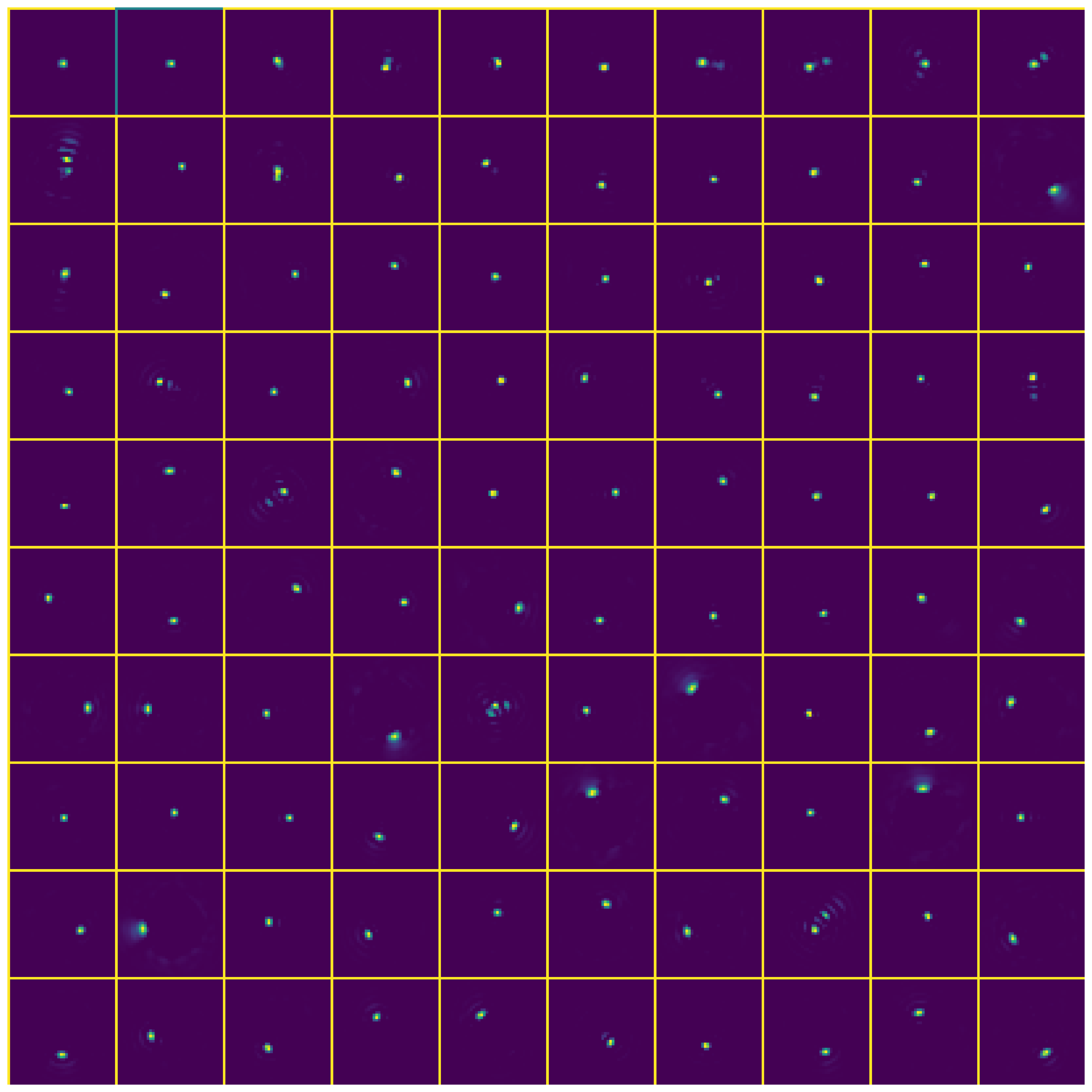
A typical NMF basis set looks like this:

1.3.3. Example
Once the basis is computed, you can carry out the deconvolution. At the moment, all objects have to share the wavelength and no diversity is alloed, but we are working on extending torchmfbd v0.1 to allow for them. The following example shows how to deconvolve a field of view with two objects without a diversity channel. The field of view is deconvolved in one single patch. First we define a configuration file that controls the general behavior of the deconvolution. This configuration file can also be defined in the code as a dictionary:
telescope:
    diameter: 100.0
    central_obscuration : 0.0

images:
    n_pixel : 128
    wavelength : 8542.0
    pix_size : 0.059
    apodization_border : 6

object1:
    wavelength : 8542.0
    image_filter: tophat
    cutoff : [0.75, 0.80]

object2:
    wavelength : 8542.0
    image_filter: tophat
    cutoff : [0.75, 0.80]

optimization:
    gpu : 0
    transform : softplus
    softplus_scale : 1000.0
    lr_obj : 0.02
    lr_tt : 0.003
    lr_modes : 0.08

regularization:
    smooth1:
        variable: tiptilt
        lambda: 0.01
    smooth2:
        variable: modes
        lambda: 0.01
    iuwt1:
        variable : object
        lambda : 0.0
        nbands : 5

psf:
    model : nmf
    nmax_modes : 150
    filename: '../basis/nmf_8542_n_150_r0_5_30.npz'
    ngrid_modes: 2

initialization:
    object : contrast
    modes_std : 0.0

annealing:
    type: none
    start_pct : 0.0
    end_pct : 0.85
The deconvolution can be carried out by the following code:
decSI = torchmfbd.DeconvolutionSV('spot_8542_nmf.yaml')

# Patchify and add the frames
for i in range(2):
    decSI.add_frames(frames[:, i, :, :, :], id_object=i, id_diversity=0, diversity=0.0)


decSI.deconvolve(simultaneous_sequences=1,
                 n_iterations=10,
                 batch_size=12)

obj = [None] * 2
for i in range(2):
    obj[i] = decSI.obj[i].cpu().numpy()

fig, ax = pl.subplots(nrows=2, ncols=2, figsize=(10, 10))
for i in range(2):
    ax[0, i].imshow(frames[0, i, 0, :, :])
    ax[1, i].imshow(obj[i][0, :, :])
First, we instantiate the torchmfbd.DeconvolutionSV class with the configuration file. We then add the frames
object by object, indicating the index of the object id_object and the index of the
diversity channel id_diversity. Note that, torchmfbd v0.1 does not yet allow for adding diversity or objects at
different wavelengths properly. In this case, we have two objects and no diversity channel, so we set id_diversity=0 and
diversity=0.0.
The deconvolution is carried out by calling the deconvolve method. The method takes several arguments:
simultaneous_sequences: The number of patches to deconvolve simultaneously. If you have plenty of VRAM, you can increase this number to speed up the deconvolution.n_iterations: The number of iterations to carry out.batch_size: The batch size to use when dealing with the bursts.
1.3.4. Output
Once the deconvolution is finished, several attributes are available in the deconvolution object:
obj: The deconvolved objects.tiptilt_lr: The spatially variant tiptilt coefficientstiptilt_hr: The spatially variant tiptilt coefficients interpolated to the full field of viewmodes_lr: The spatially variant modal coefficientsmodes_hr: The spatially variant modal coefficients interpolated to the full field of view