6.2. Synthesis with a configuration file
Perhaps the simplest approach to Hazel is to use configuration files. In this notebook we show how to use a configuration file to run Hazel in different situations.
6.2.1. Single pixel synthesis
[1]:
%matplotlib inline
import numpy as np
import matplotlib.pyplot as pl
import hazel
import h5py
print(hazel.__version__)
label = ['I', 'Q', 'U', 'V']
/scratch/miniconda3/envs/py36/lib/python3.6/site-packages/h5py/__init__.py:36: FutureWarning: Conversion of the second argument of issubdtype from `float` to `np.floating` is deprecated. In future, it will be treated as `np.float64 == np.dtype(float).type`.
  from ._conv import register_converters as _register_converters
2018.06.07
Configuration files can be used very simply by just instantiating the Model with a configuration file. First, let’s print the configuration file. The architecture of the file is explained in the documentation.
[2]:
%cat conf_single.ini
# Hazel configuration File

[Working mode]
Output file = output.h5
Number of cycles = 1

# Topology
# Always photosphere and then chromosphere
# Photospheres are only allowed to be added with a filling factor
# Atmospheres share a filling factor if they are in parenthesis
# Atmospheres are one after the other with the -> operator
# Atmosphere 1 = ph2 -> ch1 -> ch2

[Spectral regions]
    [[Region 1]]
    Name = spec1
    Wavelength = 10826, 10833, 150
    Topology = ph1 -> ch1 -> te1
    Stokes weights = 1.0, 1.0, 1.0, 1.0
    LOS = 0.0, 0.0, 90.0
    Boundary condition = 1.0, 0.0, 0.0, 0.0       # I/Ic(mu=1), Q/Ic(mu=1), U/Ic(mu=1), V/Ic(mu=1)
    Wavelength file = 'observations/10830.wavelength'
    Wavelength weight file = 'observations/10830.weights'
    Observations file = 'observations/10830_stokes.1d'
    Weights Stokes I = 1.0, 0.0, 0.0, 0.0
    Weights Stokes Q = 0.0, 0.0, 0.0, 0.0
    Weights Stokes U = 0.0, 0.0, 0.0, 0.0
    Weights Stokes V = 0.0, 0.0, 0.0, 0.0
    Mask file = None

[Atmospheres]

    [[Photosphere 1]]
    Name = ph1
    Reference atmospheric model = 'photospheres/model_photosphere_200.1d'
    Spectral region = spec1
    Wavelength = 10826, 10833
    Spectral lines = 300,

        [[[Ranges]]]
        T      = 2500.0, 9000.0
        vmic   = 0.0, 3.0
        v      = -10.0, 10.0
        Bx     = -1000.0, 1000.0
        By     = -1000.0, 1000.0
        Bz     = -1000.0, 1000.0
        ff     = 0.0, 1.001

        [[[Nodes]]]
        T      = 1, 1, 5, 5
        vmic   = 1, 0, 1, 1
        v      = 0, 0, 1, 1
        Bx     = 0, 0, 1, 1
        By     = 0, 0, 1, 1
        Bz     = 0, 0, 1, 1
        ff     = 0, 0, 0, 0


    [[Chromosphere 1]]
    Name = ch1                                              # Name of the atmosphere component
    Spectral region = spec1                                 # Spectral region to be used for synthesis
    Height = 3.0                                            # Height of the slab
    Line = 10830                                            # 10830, 5876
    Wavelength = 10828, 10833                         # Wavelength range used for synthesis
    Reference atmospheric model = 'chromospheres/model_chromosphere.1d'    # File with model parameters

        [[[Ranges]]]
        Bx     = -500, 500
        By     = -500, 500
        Bz     = -500, 500
        tau    = 0.1, 2.0
        v      = -10.0, 10.0
        deltav = 3.0, 12.0
        beta   = 0.9, 2.0
        a      = 0.0, 1.0
        ff     = 0.0, 1.001


        [[[Nodes]]]
        Bx     = 0, 0, 1, 1
        By     = 0, 0, 1, 1
        Bz     = 0, 0, 1, 1
        tau    = 0, 0, 0, 0
        v      = 0, 0, 0, 0
        deltav = 0, 0, 0, 0
        beta   = 0, 0, 0, 0
        a      = 0, 0, 0, 0
        ff     = 0, 0, 0, 0

    [[Parametric 1]]
    Name = te1
    Spectral region = spec1
    Wavelength = 10828, 10833
    Reference atmospheric model = 'telluric/model_telluric.1d'    # File with model parameters
    Type = Voigt           # Voigt, MoGaussian, MoVoigt

        [[[Ranges]]]
        Lambda0 = 10832.0, 10834.0
        Sigma = 0.1, 0.5
        Depth = 0.2, 0.8
        a = 0.0, 1.2
        ff = 0.0, 1.001

        [[[Nodes]]]
        Lambda0 = 0, 0, 0, 0
        Sigma = 0, 0, 0, 0
        Depth = 0, 0, 0, 0
        a = 0, 0, 0, 0
        ff = 0, 0, 0, 0
We use this file and do the synthesis.
[3]:
mod = hazel.Model('conf_single.ini', working_mode='synthesis', verbose=3)
mod.synthesize()
2018-09-07 08:50:49,092 - Adding spectral region spec1
2018-09-07 08:50:49,094 -   - Reading wavelength axis from observations/10830.wavelength
2018-09-07 08:50:49,097 -   - Reading wavelength weights from observations/10830.weights
2018-09-07 08:50:49,101 -   - Using observations from observations/10830_stokes.1d
2018-09-07 08:50:49,102 -   - No mask for pixels
2018-09-07 08:50:49,103 -   - Using LOS ['0.0', '0.0', '90.0']
2018-09-07 08:50:49,104 -   - Using boundary condition ['1.0', '0.0', '0.0', '0.0']
2018-09-07 08:50:49,105 - Using 1 cycles
2018-09-07 08:50:49,106 - Not using randomizations
2018-09-07 08:50:49,106 - Adding atmospheres
2018-09-07 08:50:49,107 -   - New available photosphere : ph1
2018-09-07 08:50:49,108 -     * Adding line : [300]
2018-09-07 08:50:49,109 -     * Magnetic field reference frame : vertical
2018-09-07 08:50:49,110 -     * Reading 1D model photospheres/model_photosphere_200.1d as reference
2018-09-07 08:50:49,112 -   - New available chromosphere : ch1
2018-09-07 08:50:49,113 -     * Adding line : 10830
2018-09-07 08:50:49,114 -     * Magnetic field reference frame : vertical
2018-09-07 08:50:49,115 -     * Reading 1D model chromospheres/model_chromosphere.1d as reference
2018-09-07 08:50:49,117 -   - New available parametric : te1
2018-09-07 08:50:49,118 -     * Reading 1D model telluric/model_telluric.1d as reference
2018-09-07 08:50:49,119 - Adding topologies
2018-09-07 08:50:49,120 -   - ph1 -> ch1 -> te1
2018-09-07 08:50:49,120 - Removing unused atmospheres
2018-09-07 08:50:49,121 - Number of pixels to read : 1
And now do some plots.
[4]:
f, ax = pl.subplots(nrows=2, ncols=2, figsize=(10,10))
ax = ax.flatten()
for i in range(4):
    ax[i].plot(mod.spectrum['spec1'].wavelength_axis - 10830, mod.spectrum['spec1'].stokes[i,:])

for i in range(4):
    ax[i].set_xlabel('Wavelength - 10830[$\AA$]')
    ax[i].set_ylabel('{0}/Ic'.format(label[i]))
    ax[i].set_xlim([-4,3])

pl.tight_layout()
/scratch/miniconda3/envs/py36/lib/python3.6/site-packages/matplotlib/figure.py:2267: UserWarning: This figure includes Axes that are not compatible with tight_layout, so results might be incorrect.
  warnings.warn("This figure includes Axes that are not compatible "

It is possible to save the output of a single pixel to a file. In this case, just open the file, do the synthesis, write to the file and close it.
[5]:
mod = hazel.Model('conf_single.ini', working_mode='synthesis')
mod.open_output()
mod.synthesize()
mod.write_output()
mod.close_output()
The output file contains a dataset for the currently synthesized spectral region. Here you can see the datasets and their content:
[6]:
f = h5py.File('output.h5', 'r')
print(list(f.keys()))
print(list(f['spec1'].keys()))
['spec1']
['chi2', 'stokes', 'wavelength']
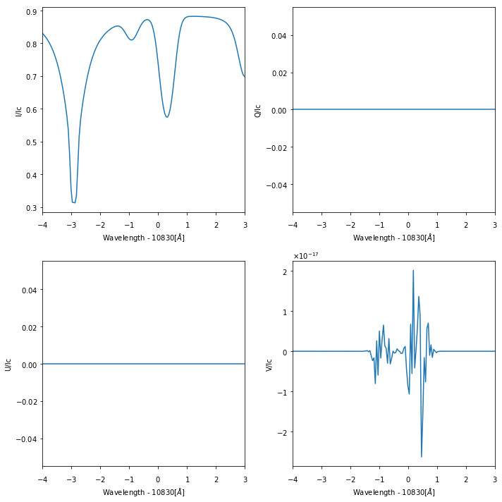
And then we do some plots:
[7]:
fig, ax = pl.subplots(nrows=2, ncols=2, figsize=(10,10))
ax = ax.flatten()
for i in range(4):
    ax[i].plot(f['spec1']['wavelength'][:] - 10830, f['spec1']['stokes'][0,0,0,i,:])

for i in range(4):
    ax[i].set_xlabel('Wavelength - 10830[$\AA$]')
    ax[i].set_ylabel('{0}/Ic'.format(label[i]))
    ax[i].set_xlim([-4,3])

pl.tight_layout()

f.close()
/scratch/miniconda3/envs/py36/lib/python3.6/site-packages/matplotlib/figure.py:2267: UserWarning: This figure includes Axes that are not compatible with tight_layout, so results might be incorrect.
  warnings.warn("This figure includes Axes that are not compatible "
6.2.2. Many pixels synthesis
Synthesizing many pixels can be exhausting and time consuming if you do it one by one. For this reason, Hazel can admit HDF5 files with different models for the synthesis.
6.2.2.1. Without MPI
The simplest option is to iterate over all pixels with a single CPU. To this end, we make use of the iterator. You first instantiate the iterator and then pass the model to the iterator, which will take care of iterating through all pixels.
[ ]:
iterator = hazel.Iterator(use_mpi=False)
rank = iterator.get_rank()
mod = hazel.Model('conf_nonmpi_syn1d.ini', working_mode='synthesis', verbose=2)
iterator.use_model(model=mod)
iterator.run_all_pixels()
2018-09-07 08:50:51,487 - Adding spectral region spec1
2018-09-07 08:50:51,489 -   - Reading wavelength axis from observations/10830.wavelength
2018-09-07 08:50:51,492 -   - Reading wavelength weights from observations/10830.weights
2018-09-07 08:50:51,496 -   - Using observations from observations/10830_stokes.1d
2018-09-07 08:50:51,497 -   - No mask for pixels
2018-09-07 08:50:51,498 -   - Using LOS ['0.0', '0.0', '90.0']
2018-09-07 08:50:51,499 -   - Using boundary condition ['1.0', '0.0', '0.0', '0.0']
2018-09-07 08:50:51,500 - Not using randomizations
2018-09-07 08:50:51,501 - Adding atmospheres
2018-09-07 08:50:51,503 -   - New available photosphere : ph1
2018-09-07 08:50:51,504 -     * Adding line : [300]
2018-09-07 08:50:51,505 -     * Magnetic field reference frame : vertical
2018-09-07 08:50:51,506 -     * Reading 3D model photospheres/model_photosphere.h5 as reference
2018-09-07 08:50:51,510 -   - New available chromosphere : ch1
2018-09-07 08:50:51,511 -     * Adding line : 10830
2018-09-07 08:50:51,512 -     * Magnetic field reference frame : vertical
2018-09-07 08:50:51,513 -     * Reading 3D model chromospheres/model_chromosphere.h5 as reference
2018-09-07 08:50:51,516 - Adding topologies
2018-09-07 08:50:51,517 -   - ph1 -> ch1
2018-09-07 08:50:51,518 - Removing unused atmospheres
2018-09-07 08:50:51,519 - Number of pixels to read : 2
100%|██████████| 2/2 [00:00<00:00, 13.89it/s]
[ ]:
f = h5py.File('output.h5', 'r')

print('(npix,ncycle,nstokes,nlambda) -> {0}'.format(f['spec1']['stokes'].shape))

fig, ax = pl.subplots(nrows=2, ncols=2, figsize=(10,10))
ax = ax.flatten()
for j in range(2):
    for i in range(4):
        ax[i].plot(f['spec1']['wavelength'][:] - 10830, f['spec1']['stokes'][j,0,0,i,:])

for i in range(4):
    ax[i].set_xlabel('Wavelength - 10830[$\AA$]')
    ax[i].set_ylabel('{0}/Ic'.format(label[i]))
    ax[i].set_xlim([-4,1])

pl.tight_layout()

f.close()
(npix,ncycle,nstokes,nlambda) -> (2, 1, 1, 4, 150)
6.2.2.2. With MPI
In case you want to synthesize large maps in a supercomputer, you can use mpi4py and run many pixels in parallel. To this end, you pass the use_mpi=True keyword to the iterator. Then, this piece of code should be called with mpiexec to run it using MPI:
mpiexec -n 10 python code.py
[ ]:
iterator = hazel.iterator(use_mpi=True)
rank = iterator.get_rank()
mod = hazel.Model('conf_mpi_synh5.ini', working_mode='synthesis', rank=rank)
iterator.use_model(model=mod)
iterator.run_all_pixels()