6.1. Synthesis in programmatic mode

6.1.1. Simple synthesis in a chromosphere

For simple calculations, like synthesizing spectral lines in simple models, Hazel v2.0 can be used in programmatic mode. For instance, let us generate a spectral window in the near-infrared and synthesize the He I 10830 A line with some parameters.

%matplotlib inline
import numpy as np
import matplotlib.pyplot as pl
import hazel
print(hazel.__version__)
label = ['I', 'Q', 'U', 'V']

1.9.0

Let’s first do a simple experiment in which we synthesize the 10830 A line for a set of parameters. Let’s first instantiating a hazel model. We set the verbosity to a high level as an example but you should lower it when doing calculations to avoid crowding your terminal:

mod = hazel.Model(working_mode='synthesis', verbose=3)

The first thing to do with the model is to add a spectral region for our synthesis.

mod.add_spectral({'Name': 'spec1', 'Wavelength': [10826, 10833, 150], 'topology': 'ch1',
    'LOS': [0.0,0.0,90.0], 'Boundary condition': [1.0,0.0,0.0,0.0]})

2018-05-07 12:35:53,388 - Adding spectral region spec1
2018-05-07 12:35:53,391 -   - Using wavelength axis from 10826.0 to 10833.0 with 150 steps
2018-05-07 12:35:53,393 -   - Not mask for pixels
2018-05-07 12:35:53,396 -   - Using LOS [0.0, 0.0, 90.0]
2018-05-07 12:35:53,398 -   - Using boundary condition [0.0, 0.0, 90.0]

Note that we need to define the angles defining the line-of-sight, the boundary condition, the wavelength range, the name and the topology. We specify in this case that the topology is just a single chromosphere that we label as ch1. We need now to define this chromosphere:

mod.add_chromosphere({'Name': 'ch1', 'Spectral region': 'spec1', 'Height': 3.0, 'Line': '10830',
                      'Wavelength': [10826, 10833]})

2018-05-07 12:35:54,348 -     * Adding line : 10830

Now that we have defined all elements of the synthesis, we finish the setup by invoking the following, which will add all topologies to the spectrum and remove unused atmospheres (if any):

mod.setup()

2018-05-07 12:35:55,146 - Adding topologies
2018-05-07 12:35:55,149 -   - ch1
2018-05-07 12:35:55,151 - Removing unused atmospheres
2018-05-07 12:35:55,152 - Number of pixels to read : 1

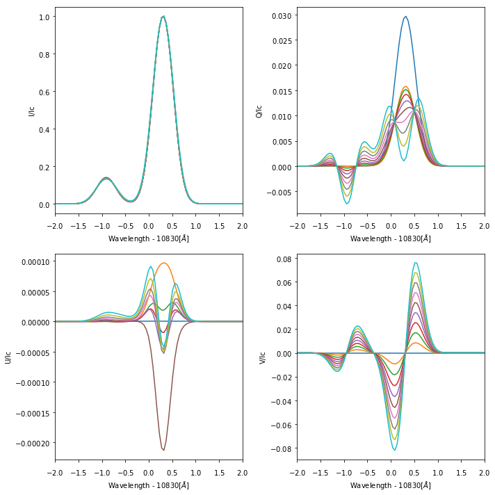
It’s time now to modify the parameters of the chromosphere and do some plots. You can have access to the wavelength axis and to the synthetic spectrum by accessing the wavelength_axisand stokes properties of mod.spectrum[name], where nameis the name given to the spectral region.

f, ax = pl.subplots(nrows=2, ncols=2, figsize=(10,10))
ax = ax.flatten()
for j in range(10):
    for i in range(4):
        mod.atmospheres['ch1'].set_parameters([50.0*j,0.0,100.0*j,0.2,0.0,8.0,1.0,0.0], 1.0)
        mod.synthesize()
        ax[i].plot(mod.spectrum['spec1'].wavelength_axis - 10830, mod.spectrum['spec1'].stokes[i,:])

for i in range(4):
    ax[i].set_xlabel('Wavelength - 10830[$\AA$]')
    ax[i].set_ylabel('{0}/Ic'.format(label[i]))
    ax[i].set_xlim([-2,2])

pl.tight_layout()

/scratch/miniconda3/envs/py36/lib/python3.6/site-packages/matplotlib/figure.py:2267: UserWarning: This figure includes Axes that are not compatible with tight_layout, so results might be incorrect.
  warnings.warn("This figure includes Axes that are not compatible "

As another example, let’s generate a profile for an off-limb observation. To this end, we just simply select \(\theta_\mathrm{obs}=90^\circ\) and set the boundary condition of intensity to zero.

mod = hazel.Model(working_mode='synthesis', verbose=True)
mod.add_spectral({'Name': 'spec1', 'Wavelength': [10826, 10833, 150], 'topology': 'ch1',
    'LOS': [90.0,0.0,90.0], 'Boundary condition': [0.0,0.0,0.0,0.0]})
mod.add_chromosphere({'Name': 'ch1', 'Spectral region': 'spec1', 'Height': 3.0, 'Line': '10830',
                      'Wavelength': [10826, 10833]})
mod.setup()

f, ax = pl.subplots(nrows=2, ncols=2, figsize=(10,10))
ax = ax.flatten()
for j in range(10):
    for i in range(4):
        mod.atmospheres['ch1'].set_parameters([50.0*j,0.0,100.0*j,0.2,0.0,8.0,1.0,0.0], 1.0)
        mod.synthesize()
        ax[i].plot(mod.spectrum['spec1'].wavelength_axis - 10830, mod.spectrum['spec1'].stokes[i,:])

for i in range(4):
    ax[i].set_xlabel('Wavelength - 10830[$\AA$]')
    ax[i].set_ylabel('{0}/Ic'.format(label[i]))
    ax[i].set_xlim([-2,2])

pl.tight_layout()

2018-05-07 12:35:08,343 - Adding spectral region spec1
2018-05-07 12:35:08,345 -   - Using wavelength axis from 10826.0 to 10833.0 with 150 steps
2018-05-07 12:35:08,346 -   - Not mask for pixels
2018-05-07 12:35:08,348 -   - Using LOS [90.0, 0.0, 90.0]
2018-05-07 12:35:08,349 -   - Using off-limb normalization (peak intensity)
2018-05-07 12:35:08,351 -   - Using boundary condition [90.0, 0.0, 90.0]
2018-05-07 12:35:08,353 -     * Adding line : 10830
2018-05-07 12:35:08,355 - Adding topologies
2018-05-07 12:35:08,357 -   - ch1
2018-05-07 12:35:08,359 - Removing unused atmospheres
2018-05-07 12:35:08,360 - Number of pixels to read : 1
/scratch/miniconda3/envs/py36/lib/python3.6/site-packages/matplotlib/figure.py:2267: UserWarning: This figure includes Axes that are not compatible with tight_layout, so results might be incorrect.
  warnings.warn("This figure includes Axes that are not compatible "

6.1.2. Synthesizing with several atmospheres

Now that we know how to compute a single atmosphere, let’s complicate things a little and add a photosphere below the chromosphere. We define again the spectral region and add a photosphere and a chromosphere. For the photosphere, it’s easier to pass a 1D model that will be automatically read and used. If not, then you would need to read the model yourself and change the parameters. The file contents follows:

%cat photospheres/model_photosphere.1d

ff
1.0

  logtau     T        Pe           vmic        v            Bx           By         Bz
  1.2000   8879.7  2.99831E+03  0.000E+00  0.0000E+00   5.0000E+02    0.0000E+00  0.0000E+00
  1.1000   8720.2  2.46927E+03  0.000E+00  0.0000E+00   5.0000E+02    0.0000E+00  0.0000E+00
  1.0000   8551.0  1.98933E+03  0.000E+00  0.0000E+00   5.0000E+02    0.0000E+00  0.0000E+00
  0.9000   8372.2  1.56782E+03  0.000E+00  0.0000E+00   5.0000E+02    0.0000E+00  0.0000E+00
  0.8000   8183.7  1.20874E+03  0.000E+00  0.0000E+00   5.0000E+02    0.0000E+00  0.0000E+00
  0.7000   7985.6  9.11633E+02  0.000E+00  0.0000E+00   5.0000E+02    0.0000E+00  0.0000E+00
  0.6000   7777.9  6.72597E+02  0.000E+00  0.0000E+00   5.0000E+02    0.0000E+00  0.0000E+00
  0.5000   7557.6  4.75281E+02  0.000E+00  0.0000E+00   5.0000E+02    0.0000E+00  0.0000E+00
  0.4000   7326.3  3.25088E+02  0.000E+00  0.0000E+00   5.0000E+02    0.0000E+00  0.0000E+00
  0.3000   7083.8  2.15232E+02  0.000E+00  0.0000E+00   5.0000E+02    0.0000E+00  0.0000E+00
  0.2000   6860.1  1.43137E+02  0.000E+00  0.0000E+00   5.0000E+02    0.0000E+00  0.0000E+00
  0.1000   6640.1  9.38622E+01  0.000E+00  0.0000E+00   5.0000E+02    0.0000E+00  0.0000E+00
  0.0000   6424.0  6.06914E+01  0.000E+00  0.0000E+00   5.0000E+02    0.0000E+00  0.0000E+00
 -0.1000   6239.3  4.15733E+01  0.000E+00  0.0000E+00   5.0000E+02    0.0000E+00  0.0000E+00
 -0.2000   6072.2  2.91055E+01  0.000E+00  0.0000E+00   5.0000E+02    0.0000E+00  0.0000E+00
 -0.3000   5922.8  2.08261E+01  0.000E+00  0.0000E+00   5.0000E+02    0.0000E+00  0.0000E+00
 -0.4000   5777.8  1.53184E+01  0.000E+00  0.0000E+00   5.0000E+02    0.0000E+00  0.0000E+00
 -0.5000   5643.8  1.15489E+01  0.000E+00  0.0000E+00   5.0000E+02    0.0000E+00  0.0000E+00
 -0.6000   5520.8  8.92457E+00  0.000E+00  0.0000E+00   5.0000E+02    0.0000E+00  0.0000E+00
 -0.7000   5409.8  7.08599E+00  0.000E+00  0.0000E+00   5.0000E+02    0.0000E+00  0.0000E+00
 -0.8000   5310.4  5.77373E+00  0.000E+00  0.0000E+00   5.0000E+02    0.0000E+00  0.0000E+00
 -0.9000   5222.4  4.82788E+00  0.000E+00  0.0000E+00   5.0000E+02    0.0000E+00  0.0000E+00
 -1.0000   5140.4  4.03386E+00  0.000E+00  0.0000E+00   5.0000E+02    0.0000E+00  0.0000E+00
 -1.1000   5067.0  3.41302E+00  0.000E+00  0.0000E+00   5.0000E+02    0.0000E+00  0.0000E+00
 -1.2000   5002.4  2.92422E+00  0.000E+00  0.0000E+00   5.0000E+02    0.0000E+00  0.0000E+00
 -1.3000   4937.5  2.49379E+00  0.000E+00  0.0000E+00   5.0000E+02    0.0000E+00  0.0000E+00
 -1.4000   4876.8  2.13513E+00  0.000E+00  0.0000E+00   5.0000E+02    0.0000E+00  0.0000E+00
 -1.5000   4820.4  1.83529E+00  0.000E+00  0.0000E+00   5.0000E+02    0.0000E+00  0.0000E+00
 -1.6000   4765.7  1.57718E+00  0.000E+00  0.0000E+00   5.0000E+02    0.0000E+00  0.0000E+00
 -1.7000   4714.0  1.35790E+00  0.000E+00  0.0000E+00   5.0000E+02    0.0000E+00  0.0000E+00
 -1.8000   4665.2  1.17127E+00  0.000E+00  0.0000E+00   5.0000E+02    0.0000E+00  0.0000E+00
 -1.9000   4617.4  1.01011E+00  0.000E+00  0.0000E+00   5.0000E+02    0.0000E+00  0.0000E+00
 -2.0000   4571.7  8.71864E-01  0.000E+00  0.0000E+00   5.0000E+02    0.0000E+00  0.0000E+00
 -2.1000   4527.9  7.53168E-01  0.000E+00  0.0000E+00   5.0000E+02    0.0000E+00  0.0000E+00
 -2.2000   4485.7  6.50980E-01  0.000E+00  0.0000E+00   5.0000E+02    0.0000E+00  0.0000E+00
 -2.3000   4445.3  5.63044E-01  0.000E+00  0.0000E+00   5.0000E+02    0.0000E+00  0.0000E+00
 -2.4000   4406.6  4.87321E-01  0.000E+00  0.0000E+00   5.0000E+02    0.0000E+00  0.0000E+00
 -2.5000   4369.9  4.22256E-01  0.000E+00  0.0000E+00   5.0000E+02    0.0000E+00  0.0000E+00
 -2.6000   4335.0  3.66210E-01  0.000E+00  0.0000E+00   5.0000E+02    0.0000E+00  0.0000E+00
 -2.7000   4302.0  3.17890E-01  0.000E+00  0.0000E+00   5.0000E+02    0.0000E+00  0.0000E+00
 -2.8000   4271.8  2.76597E-01  0.000E+00  0.0000E+00   5.0000E+02    0.0000E+00  0.0000E+00
 -2.9000   4243.9  2.41060E-01  0.000E+00  0.0000E+00   5.0000E+02    0.0000E+00  0.0000E+00
 -3.0000   4218.4  2.10432E-01  0.000E+00  0.0000E+00   5.0000E+02    0.0000E+00  0.0000E+00
 -3.1000   4199.1  1.84897E-01  0.000E+00  0.0000E+00   5.0000E+02    0.0000E+00  0.0000E+00
 -3.2000   4184.1  1.63125E-01  0.000E+00  0.0000E+00   5.0000E+02    0.0000E+00  0.0000E+00
 -3.3000   4173.3  1.44504E-01  0.000E+00  0.0000E+00   5.0000E+02    0.0000E+00  0.0000E+00
 -3.4000   4169.3  1.28638E-01  0.000E+00  0.0000E+00   5.0000E+02    0.0000E+00  0.0000E+00
 -3.5000   4170.8  1.15030E-01  0.000E+00  0.0000E+00   5.0000E+02    0.0000E+00  0.0000E+00
 -3.6000   4177.9  1.03325E-01  0.000E+00  0.0000E+00   5.0000E+02    0.0000E+00  0.0000E+00
 -3.7000   4194.8  9.26851E-02  0.000E+00  0.0000E+00   5.0000E+02    0.0000E+00  0.0000E+00
 -3.8000   4219.3  8.32714E-02  0.000E+00  0.0000E+00   5.0000E+02    0.0000E+00  0.0000E+00
 -3.9000   4251.5  7.49313E-02  0.000E+00  0.0000E+00   5.0000E+02    0.0000E+00  0.0000E+00
 -4.0000   4309.5  6.58077E-02  0.000E+00  0.0000E+00   5.0000E+02    0.0000E+00  0.0000E+00
 -4.1000   4384.3  5.71418E-02  0.000E+00  0.0000E+00   5.0000E+02    0.0000E+00  0.0000E+00
 -4.2000   4475.8  4.90563E-02  0.000E+00  0.0000E+00   5.0000E+02    0.0000E+00  0.0000E+00
 -4.3000   4632.6  5.07160E-02  0.000E+00  0.0000E+00   5.0000E+02    0.0000E+00  0.0000E+00
 -4.4000   4830.3  5.72114E-02  0.000E+00  0.0000E+00   5.0000E+02    0.0000E+00  0.0000E+00
 -4.5000   5069.1  7.04217E-02  0.000E+00  0.0000E+00   5.0000E+02    0.0000E+00  0.0000E+00
 -4.6000   5261.7  8.84299E-02  0.000E+00  0.0000E+00   5.0000E+02    0.0000E+00  0.0000E+00
 -4.7000   5451.7  1.17157E-01  0.000E+00  0.0000E+00   5.0000E+02    0.0000E+00  0.0000E+00
 -4.8000   5639.2  1.63763E-01  0.000E+00  0.0000E+00   5.0000E+02    0.0000E+00  0.0000E+00
 -4.9000   5779.7  1.85029E-01  0.000E+00  0.0000E+00   5.0000E+02    0.0000E+00  0.0000E+00
 -5.0000   5895.5  1.93060E-01  0.000E+00  0.0000E+00   5.0000E+02    0.0000E+00  0.0000E+00
 -5.1000   5986.5  1.86025E-01  0.000E+00  0.0000E+00   5.0000E+02    0.0000E+00  0.0000E+00
 -5.2000   6078.6  1.78837E-01  0.000E+00  0.0000E+00   5.0000E+02    0.0000E+00  0.0000E+00
 -5.3000   6158.9  1.65029E-01  0.000E+00  0.0000E+00   5.0000E+02    0.0000E+00  0.0000E+00
 -5.4000   6227.4  1.46178E-01  0.000E+00  0.0000E+00   5.0000E+02    0.0000E+00  0.0000E+00
 -5.5000   6300.0  1.33777E-01  0.000E+00  0.0000E+00   5.0000E+02    0.0000E+00  0.0000E+00
 -5.6000   6368.8  1.21921E-01  0.000E+00  0.0000E+00   5.0000E+02    0.0000E+00  0.0000E+00
 -5.7000   6433.7  1.10655E-01  0.000E+00  0.0000E+00   5.0000E+02    0.0000E+00  0.0000E+00
 -5.8000   6525.9  1.07495E-01  0.000E+00  0.0000E+00   5.0000E+02    0.0000E+00  0.0000E+00
 -5.9000   6629.7  1.07811E-01  0.000E+00  0.0000E+00   5.0000E+02    0.0000E+00  0.0000E+00
 -6.0000   6745.3  1.11634E-01  0.000E+00  0.0000E+00   5.0000E+02    0.0000E+00  0.0000E+00

mod = hazel.Model(working_mode='synthesis', verbose=True)
mod.add_spectral({'Name': 'spec1', 'Wavelength': [10826, 10833, 150], 'topology': 'ph1->ch1',
    'LOS': [0.0,0.0,90.0], 'Boundary condition': [1.0,0.0,0.0,0.0]})
mod.add_chromosphere({'Name': 'ch1', 'Spectral region': 'spec1', 'Height': 3.0, 'Line': '10830',
                      'Wavelength': [10826, 10833]})
mod.add_photosphere({'Name': 'ph1', 'Spectral region': 'spec1', 'Spectral lines': [300],
                      'Wavelength': [10826, 10833], 'Reference atmospheric model': 'model_photosphere.1d'})
mod.setup()

2018-05-03 12:38:22,043 - Adding spectral region spec1
2018-05-03 12:38:22,045 -   - Using wavelength axis from 10826.0 to 10833.0 with 150 steps
2018-05-03 12:38:22,047 -   - Not mask for pixels
2018-05-03 12:38:22,049 -   - Using LOS [0.0, 0.0, 90.0]
2018-05-03 12:38:22,051 -   - Using boundary condition [0.0, 0.0, 90.0]
2018-05-03 12:38:22,053 -     * Adding line : 10830
2018-05-03 12:38:22,058 -     * Adding line : [300]
2018-05-03 12:38:22,063 -     * Reading 1D model model_photosphere.1d as reference
2018-05-03 12:38:22,073 - Adding topologies
2018-05-03 12:38:22,075 -   - ph1->ch1
2018-05-03 12:38:22,077 - Removing unused atmospheres
2018-05-03 12:38:22,078 - Number of pixels to read : 1

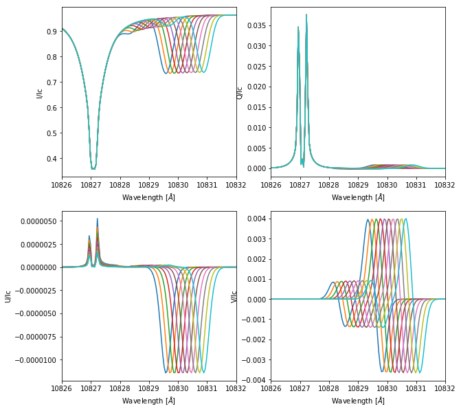
And then do the plots again by changing the velocity of the chromospheric component.

f, ax = pl.subplots(nrows=2, ncols=2, figsize=(10,10))
ax = ax.flatten()
for j in range(10):
    for i in range(4):
        mod.atmospheres['ch1'].set_parameters([50.0,0.0,100.0,0.5,-20.0+4*j,8.0,1.0,0.0], 1.0)
        mod.synthesize()
        ax[i].plot(mod.spectrum['spec1'].wavelength_axis, mod.spectrum['spec1'].stokes[i,:])

for i in range(4):
    ax[i].set_xlabel('Wavelength [$\AA$]')
    ax[i].set_ylabel('{0}/Ic'.format(label[i]))
    ax[i].set_xlim([10826,10832])

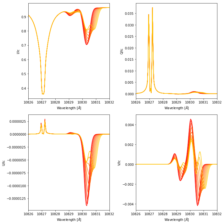
6.1.3. Synthesizing with several chromospheres

Chromospheres (and atmospheres in general) in Hazel can be combined with filling factors (using +) or as stacked atmospheres (using ->). We provide a few examples of that.

6.1.3.1. One atmosphere on top of the other

Let’s stack two chromospheres together with a photosphere below.

mod = hazel.Model(working_mode='synthesis', verbose=True)
mod.add_spectral({'Name': 'spec1', 'Wavelength': [10826, 10833, 150], 'topology': 'ph1->ch1->ch2',
    'LOS': [0.0,0.0,90.0], 'Boundary condition': [1.0,0.0,0.0,0.0]})
mod.add_chromosphere({'Name': 'ch1', 'Spectral region': 'spec1', 'Height': 3.0, 'Line': '10830',
                      'Wavelength': [10826, 10833]})
mod.add_chromosphere({'Name': 'ch2', 'Spectral region': 'spec1', 'Height': 3.0, 'Line': '10830',
                      'Wavelength': [10826, 10833]})
mod.add_photosphere({'Name': 'ph1', 'Spectral region': 'spec1', 'Spectral lines': [300],
                      'Wavelength': [10826, 10833], 'Reference atmospheric model': 'model_photosphere.1d'})
mod.setup()

2018-05-03 12:40:40,531 - Adding spectral region spec1
2018-05-03 12:40:40,532 -   - Using wavelength axis from 10826.0 to 10833.0 with 150 steps
2018-05-03 12:40:40,535 -   - Not mask for pixels
2018-05-03 12:40:40,537 -   - Using LOS [0.0, 0.0, 90.0]
2018-05-03 12:40:40,538 -   - Using boundary condition [0.0, 0.0, 90.0]
2018-05-03 12:40:40,540 -     * Adding line : 10830
2018-05-03 12:40:40,542 -     * Adding line : 10830
2018-05-03 12:40:40,544 -     * Adding line : [300]
2018-05-03 12:40:40,547 -     * Reading 1D model model_photosphere.1d as reference
2018-05-03 12:40:40,551 - Adding topologies
2018-05-03 12:40:40,553 -   - ph1->ch1->ch2
2018-05-03 12:40:40,554 - Removing unused atmospheres
2018-05-03 12:40:40,556 - Number of pixels to read : 1

Now we synthesize the emergent Stokes parameters by changing the velocity of the second component.

f, ax = pl.subplots(nrows=2, ncols=2, figsize=(10,10))
ax = ax.flatten()
for j in range(9):
#    Bx, By, Bz, tau, v, delta, beta, a
    mod.atmospheres['ch1'].set_parameters([50.0,0.0,100.0,0.3,0.0,8.0,1.0,0.0], 1.0)
    mod.atmospheres['ch2'].set_parameters([50.0,0.0,100.0,0.3,2*j,8.0,1.0,0.0], 1.0)
    mod.synthesize()
    for i in range(4):
        ax[i].plot(mod.spectrum['spec1'].wavelength_axis, mod.spectrum['spec1'].stokes[i,:], color=pl.cm.autumn(25*j))

for i in range(4):
    ax[i].set_xlabel('Wavelength [$\AA$]')
    ax[i].set_ylabel('{0}/Ic'.format(label[i]))
    ax[i].set_xlim([10826,10832])
pl.tight_layout()

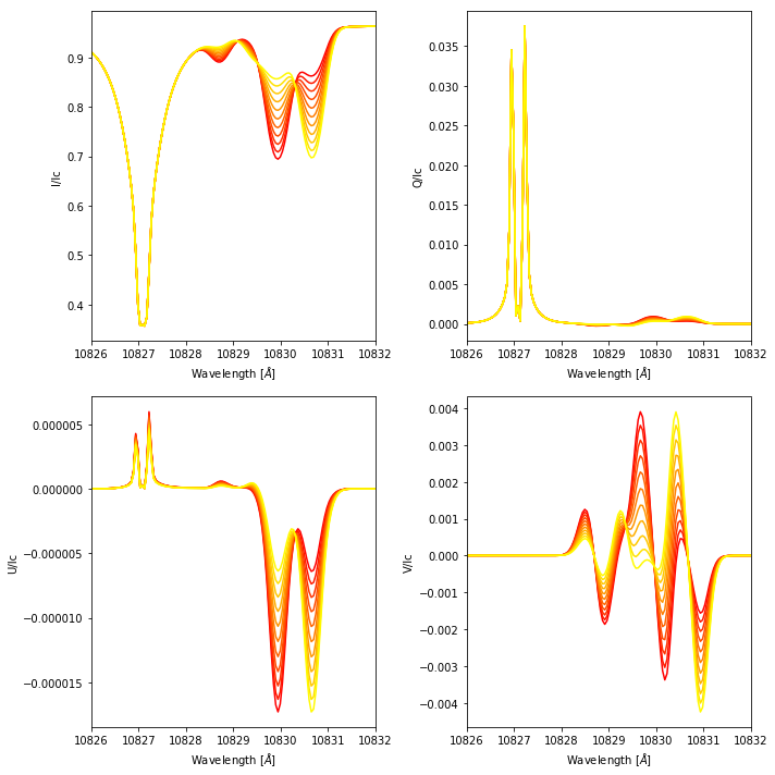
6.1.3.2. Atmospheres with filling factors

And now we combine the atmospheres with a filling factor.

mod = hazel.Model(working_mode='synthesis', verbose=True)
mod.add_spectral({'Name': 'spec1', 'Wavelength': [10826, 10833, 150], 'topology': 'ph1->ch1+ch2',
    'LOS': [0.0,0.0,90.0], 'Boundary condition': [1.0,0.0,0.0,0.0]})
mod.add_chromosphere({'Name': 'ch1', 'Spectral region': 'spec1', 'Height': 3.0, 'Line': '10830',
                      'Wavelength': [10826, 10833]})
mod.add_chromosphere({'Name': 'ch2', 'Spectral region': 'spec1', 'Height': 3.0, 'Line': '10830',
                      'Wavelength': [10826, 10833]})
mod.add_photosphere({'Name': 'ph1', 'Spectral region': 'spec1', 'Spectral lines': [300],
                      'Wavelength': [10826, 10833], 'Reference atmospheric model': 'model_photosphere.1d'})
mod.setup()

2018-05-03 12:41:41,841 - Adding spectral region spec1
2018-05-03 12:41:41,844 -   - Using wavelength axis from 10826.0 to 10833.0 with 150 steps
2018-05-03 12:41:41,848 -   - Not mask for pixels
2018-05-03 12:41:41,852 -   - Using LOS [0.0, 0.0, 90.0]
2018-05-03 12:41:41,853 -   - Using boundary condition [0.0, 0.0, 90.0]
2018-05-03 12:41:41,855 -     * Adding line : 10830
2018-05-03 12:41:41,856 -     * Adding line : 10830
2018-05-03 12:41:41,858 -     * Adding line : [300]
2018-05-03 12:41:41,859 -     * Reading 1D model model_photosphere.1d as reference
2018-05-03 12:41:41,863 - Adding topologies
2018-05-03 12:41:41,864 -   - ph1->ch1+ch2
2018-05-03 12:41:41,866 - Removing unused atmospheres
2018-05-03 12:41:41,868 - Number of pixels to read : 1

Note that filling factors will be combined so that they add up to 1. This way, it is unnecessary to set them by hand to add to 1, it is automatically done by the code. We combine two atmospheres with different velocities and we gradually change the filling factor from 0 to 1.

f, ax = pl.subplots(nrows=2, ncols=2, figsize=(10,10))
ax = ax.flatten()
for j in range(11):
#    Bx, By, Bz, tau, v, delta, beta, a
    mod.atmospheres['ch1'].set_parameters([50.0,0.0,100.0,1.0,10.0,8.0,1.0,0.0], j/10.0)
    mod.atmospheres['ch2'].set_parameters([50.0,0.0,100.0,1.0,-10.0,8.0,1.0,0.0], 1.0-j/10.0)
    mod.synthesize()
    for i in range(4):
        ax[i].plot(mod.spectrum['spec1'].wavelength_axis, mod.spectrum['spec1'].stokes[i,:], color=pl.cm.autumn(25*j))

for i in range(4):
    ax[i].set_xlabel('Wavelength [$\AA$]')
    ax[i].set_ylabel('{0}/Ic'.format(label[i]))
    ax[i].set_xlim([10826,10832])
pl.tight_layout()